How to filter in Google Sheets

The moment I see a spreadsheet filled from corner to corner with numbers, my eyes glaze over. That much data makes it nearly impossible to scan for the information I need, let alone make sense of anything. 

Which is why filters in Google Sheets are so useful—they help you focus on only the information you need. 

Here’s the short version of how to filter in Google Sheets (keep scrolling for detailed instructions).

1. Add column headers to the first row of your spreadsheet. 

2. Click any cell or highlight the specific columns you want to add a filter to. 

3. Right-click your selection, and then select Create a filter. Or click the Create a filter icon in your toolbar. 

4. A filter icon will appear next to every column heading that you’ve applied a filter to. 

5. Click the icon to filter your spreadsheet. 

Table of contents: 

What is a filter in Google Sheets

A filter in Google Sheets allows you to show specific rows of data based on cell values within a given column. 

Let’s take this simple project management tracker as an example. It’s filled with details like client name, project type, and amount billed. 

If I want to focus only on clients that have billed for more than $1,000, I can add a filter to the Amount Billed column and tell Google Sheets to show only rows where the value is $1,000 or more.

When using a column filter, you can filter only for cell values that exist within that column. For example, I can’t use the Amount Billed filter to filter for proofreading projects. I’d have to use the Project Type filter to do that. 

How to filter in Google Sheets

For this tutorial, let’s continue using our project management tracker. 

How to create a filter in Google Sheets

Before you create a filter in Google Sheets, be sure to add headings to the first row of every column—the first row of data isn’t included when you filter your data, so you want to be sure that all the data you might want to filter later on starts at row 2 or below.

Now you’re ready to create a filter. There are a few ways to do this.

Option 1: Use the toolbar 

1. Highlight the columns you want to add a filter to. You can also click any cell within the spreadsheet to automatically apply a filter to every column with data. 

2. Click the Create a filter icon in the toolbar. If the icon isn’t visible to you, first click the More icon, which looks like three dots stacked horizontally (⋮), to expand your toolbar. 

Option 2: Use the right-click menu 

1. Click any cell or highlight the specific columns you want to add a filter to. 

2. Right-click your selection, and then select Create a filter. 

Option 3: Use the Data menu 

1. Click any cell or highlight the specific columns you want to add a filter to. 

2. Click Data, and then select Create a filter. 

Regardless of the tool you use, a filter icon will appear next to every column heading that you’ve applied a filter to. 

You can repeat any of the options listed above to turn off filters—the only difference for the right-click or Data menu is that you’ll select Remove filter instead. 

How to use filters in Google Sheets 

There are two main ways to use filters in Google Sheets:

To demonstrate how to use them both, we’re going to filter our spreadsheet by Project Type to view only Proofreading projects done in 2024. 

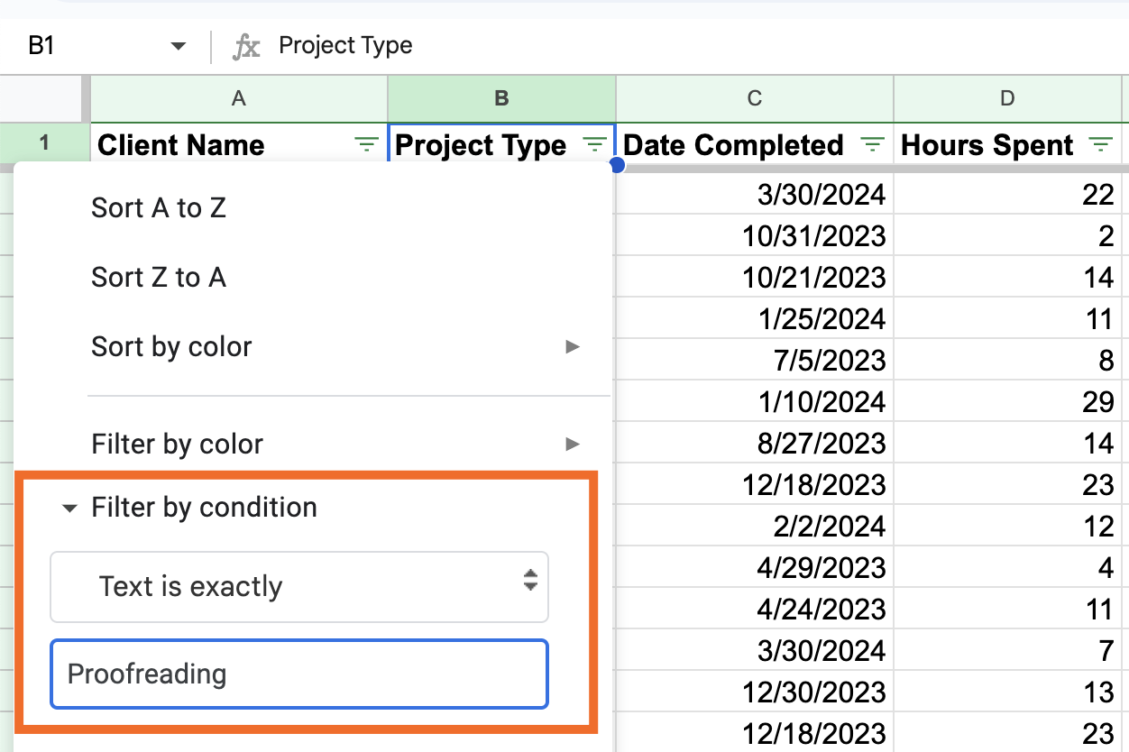
How to filter by condition in Google Sheets

1. In the Project Type column, click the filter icon. 

2. Click Filter by condition and select Text is exactly. This tells Google Sheets to display only cells containing a specific value. 

3. Enter Proofreading as the value you want Google Sheets to search for. 

   

4. Click OK. 

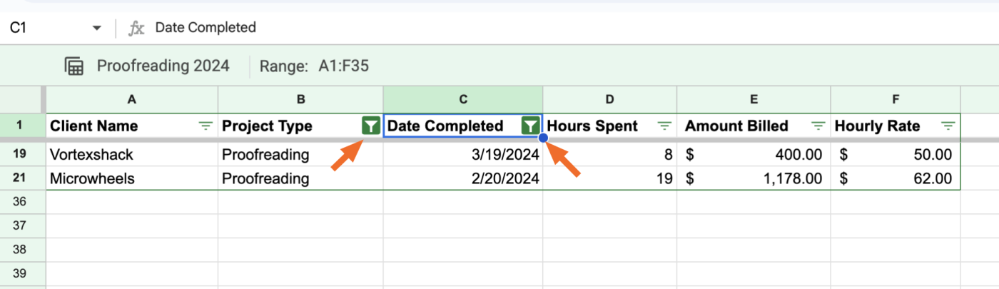
5. Repeat the same thing for the Date Completed column, but change the condition to Date is after, and choose exact date. 

6. Enter 12/31/2023. This tells Google Sheets to display only cells containing dates after December 31, 2023. 

7. Click OK. 

8. The column’s filter icon will turn into a funnel within a square to indicate that you’re looking at a filtered view of the data. 

   

It’s worth noting that there are a handful of conditions you could apply to get similar filtered results. For example, you could use Text contains or Text starts with to filter only for Proofreading projects. Similarly, you could use Greater than 12/31/2023 to filter for projects completed after December 31, 2023. 

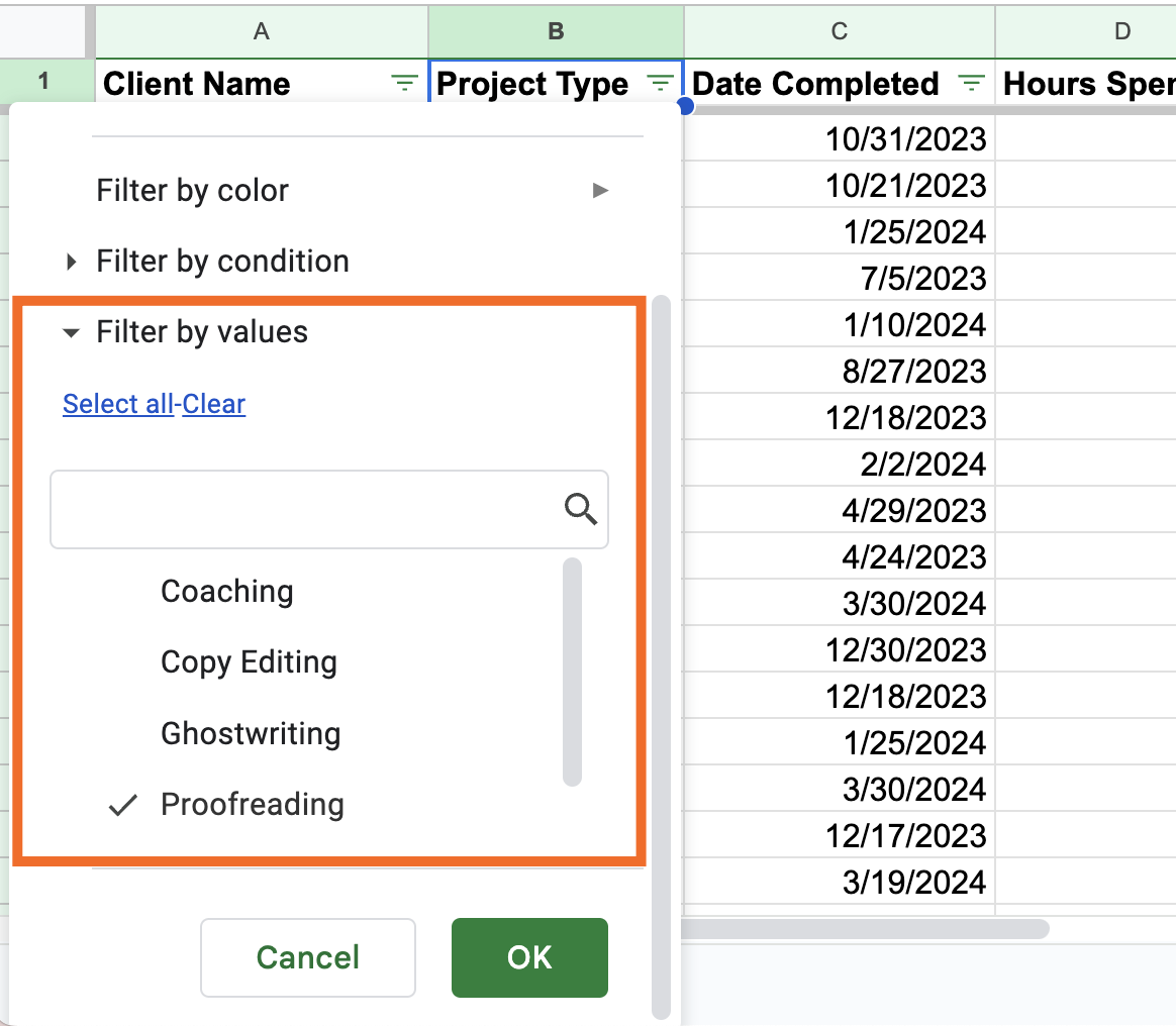
How to filter by values in Google Sheets

Filter by values lets you essentially filter by condition—the condition being Text is exactly.

1. In the column that you want to sort, click the filter icon.

2. By default, every unique value in that column is listed and selected to display. Click Clear to deselect everything. 

3. Click the value or values you want to filter for. 

4. Click OK. 

   

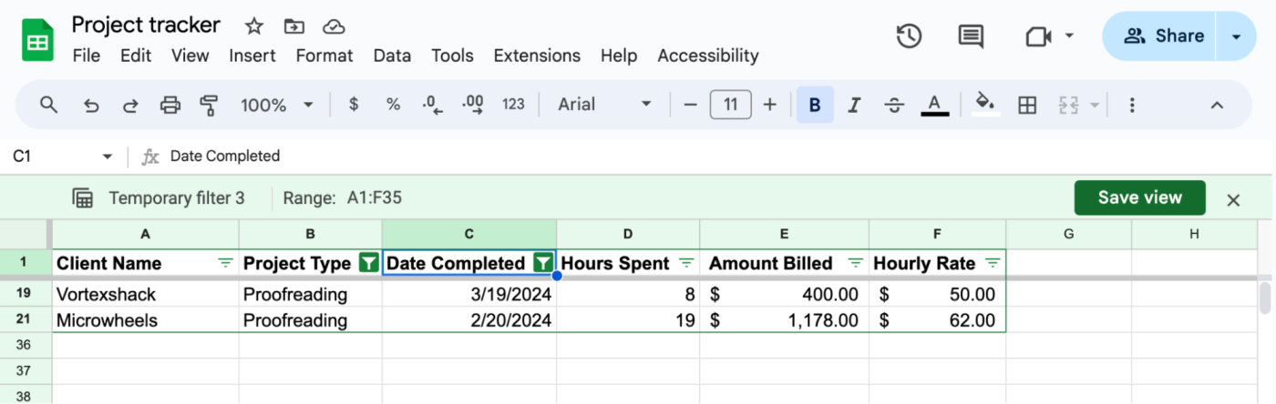
How to create a filter view in Google Sheets

A filter view in Google Sheets allows you to apply filters to only your view of a shared spreadsheet. Here’s how to create your own—you can create as many as you want. 

Note: Users with View permissions can create only a temporary filter—it won’t be saved and can’t be shared with others. 

1. Click any cell or highlight the specific columns you want to add a filter view to. 

2. Click Data, and then select Create filter view. 

3. Filter the data as you normally would. 

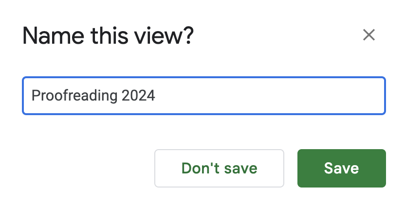
4. To save your filters, click Save view. 

   

5. Give your view a descriptive name. 

6. Click Save. 

That’s it. If you’ve already added filters to the original spreadsheet, you can also save it as a filtered view after the fact. 

1. Click Data, and then select Save as filter view. 

2. Give your view a name. 

3. Click Save.

   

How to switch filter views in Google Sheets

Need to toggle between filter views?

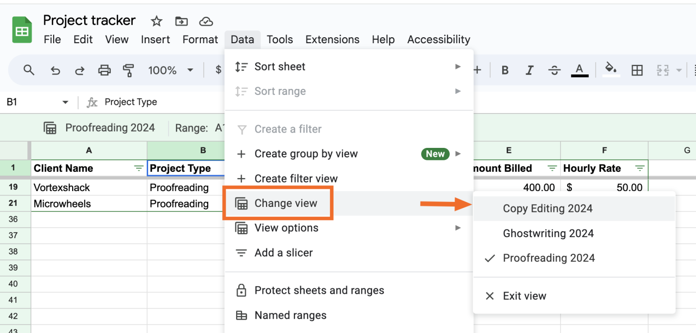
1. Click Data, and then select Change view. 

2. Select the filter view you want to switch to. 

   

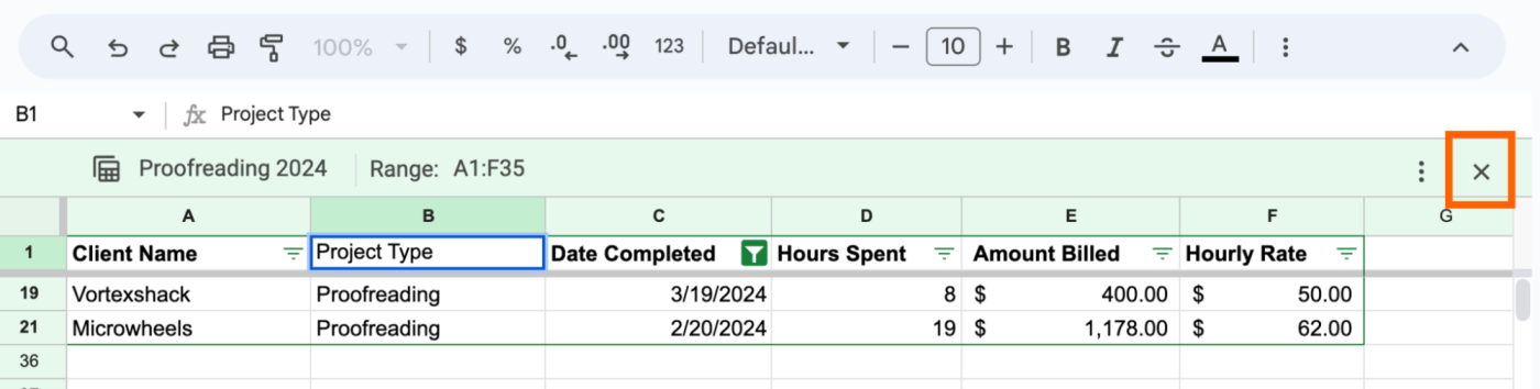
3. To exit a filtered view, click X above your spreadsheet. 

   

How to delete a filter view in Google Sheets

Far be it from me to tell Google how to do things, but I’m going to do it anyway. Deleting a filter view in Google Sheets is way too hard. Here’s how to do it. 

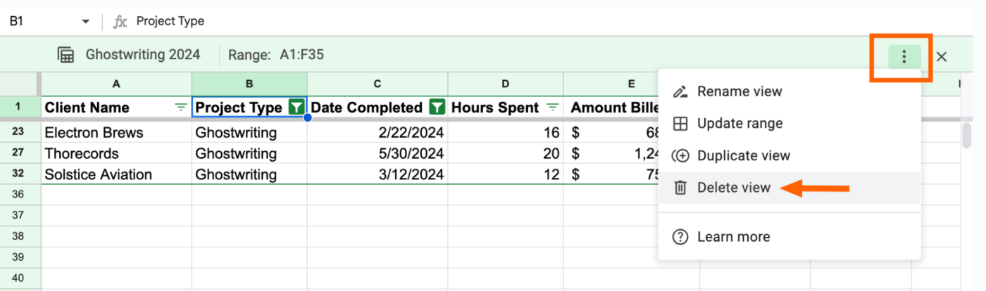
1. Click Data > Change view > Select the filter view you want to delete. 

2. Click the Options icon, which looks like three dots stacked horizontally (⋮), above your spreadsheet. 

3. Click Delete view. 

   

You’ll have to repeat the process for each view that you want to delete. Why Google didn’t add an X option next to each view in the list of filter views is beyond me. 

If you want to delete all your filter views at once, it’s much easier.

1. Click Data. 

2. Click View options, and then select Delete all views in tab. 

   

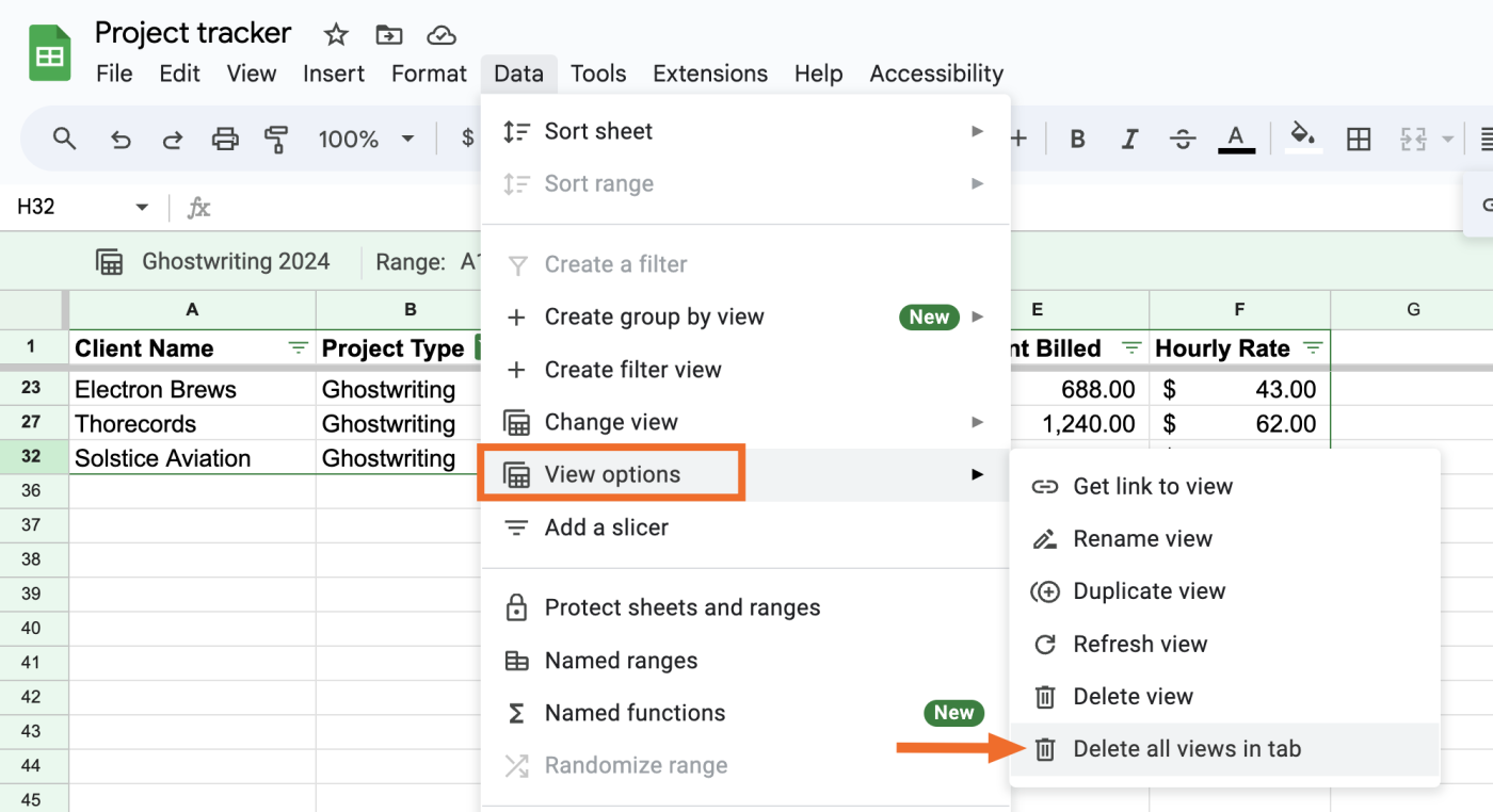
Unlike a lot of other delete actions in Google apps, Google Sheets won’t ask if you’re sure if you want to delete filter views—it’ll get straight to it. Keep this in mind before you delete any views with complex filters. 

How to share a filter view in Google Sheets 

Here’s the easiest way to share a filter view in Google Sheets. 

1. Switch to the filter view you want to share. 

2. Copy the URL in your browser’s address bar. 

3. Share the link as you normally would. 

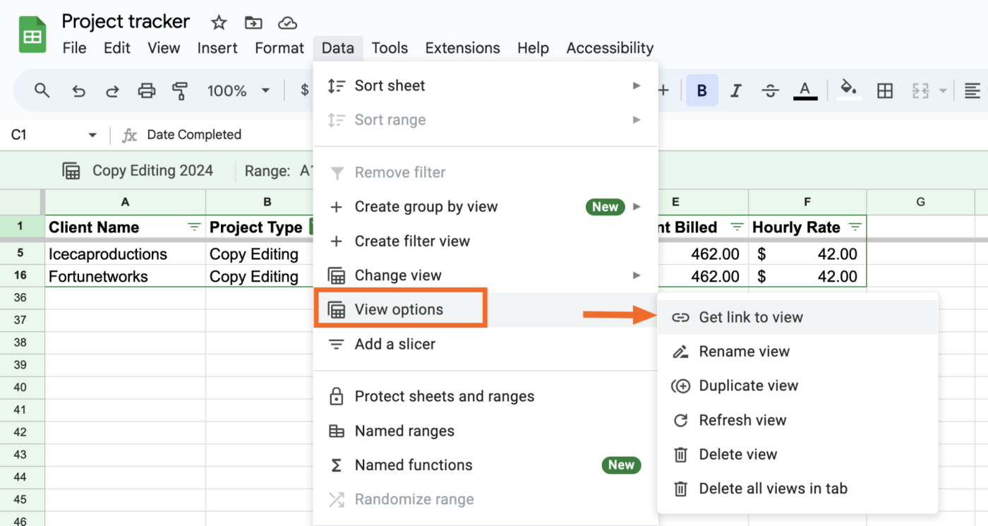
If you want to add a few extra clicks to your workflow, here’s another way.

1. Switch to the filter view you want to share. 

2. Click Data > View options > Get link to view. 

3. Share the link as you normally would. 

   

Automate Google Sheets 

Google Sheets is a great app for storing and making sense of data—but you have to first get all that data into your spreadsheet. With Zapier’s Google Sheets integration, you can automate this process and keep your data up to date across apps. Learn more about how to automate Google Sheets, or get started with one of these premade workflows.

Related reading: 

This article was originally published in May 2019 by Justin Pot. The most recent update was in July 2024.