I have a confession: I don’t really understand Mountain Time, and at this point, I’m too afraid to ask. I tend just to ask remote coworkers what time it is there—every single time I see them. (Denver team, if you’re reading this: I’m very sorry.)
Unfortunately, the same approach doesn’t work in Excel, and failure to convert time successfully can be a financial hazard. So, if you’re working with times in your next spreadsheet—time values, time zones, or otherwise—it’s important to learn how to calculate time differences in Excel.
The clock’s ticking (they have clocks in Mountain Time, right?)—so let’s get to it.
Table of contents:
Understanding time values in Excel
Excel handles time values as fractions of a 24-hour day. If the whole day is represented as the number 1, different times of the day are decimals. For example, 3:00 p.m. would be represented as 0.625 because it’s 62.5% of the way through the day (15 out of 24 hours or 15/24 = 0.625)
With me so far?
Regardless of the time you entered and whether you entered it as a decimal or a time, it’s always a decimal on the back end. Excel can display something labeled as a “time” value in the more familiar hh:mm:ss format, but it exists as a decimal.
So always set the cell type to “Time”—and if you see a weird decimal in a place where you put a time, don’t worry about it.
Basic time difference calculation
First, the most basic and most important of the calculations: a basic time difference conversion. This can be helpful for things like calculating the number of hours worked or the number of hours between you and Denver.
-
Open your Excel sheet, and add the start and end times for an activity. For the purposes of this exercise, we’ll say it’s hours clocked in and out.

-
Once you have your hours entered, copy the formula
=[End time] - [Start time]into the formula bar for the cell you want to populate with the answer. -
Replace the
[End time]and[Start time]with the values for the cells you want to use in the formula. For example, here we’ll use B2 and A2.
-
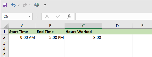
Just hit Enter, and ta-da—the number of hours worked will change automatically based on the start and end times you entered.
-
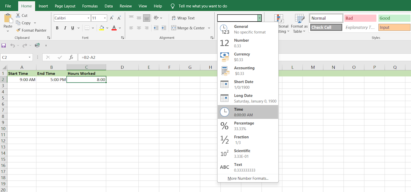
Make sure you set the cell category for the formula cell to “Time” (in this case, that would be C2). You can do that by going to the Cell Category dropdown menu and selecting the value Time. (You can do this before or after adding the formula.)
Calculating time difference across different days
A basic time difference calculation is all well and good, but what if those times are on different days? There’s a different calculation for that. To calculate the time difference across different days, follow these steps instead.
-
Open your Excel sheet, and add the start and end times for an activity. Again, for the purposes of this exercise, we’ll say it’s hours clocked in and out.

-
Then, instead of immediately adding a formula, change the cell format for all the cells. In the Format Cells dialog box in the top menu, go to the Number tab, select Custom, and use the custom format, m/d/yyyy h:mm.

This will change your cell appearance to look something like this:

You can now change both the time and date for A2 and B2. Now that we have values for each, we can calculate the time difference between cells with different times and dates.
-
For this example, copy the formula
=(End date & time - Start date & time)*24into C2. In this example, it would be=(B2-A2)*24. -
Hit Enter. The field will set to 00:00.
-
Next, change the format on that cell to Number. This will reveal the difference in hours between the two times on different days. You may note that this is not a “Time” value—that’s because we’re calculating a number of hours, not a time of day.

Tip: Always remember to check the cell formatting if your time isn’t displaying correctly.
Advanced time difference calculations
Here are some more advanced formulas that might come in handy when you’re working on specific use cases.
Handling negative time values
If you want to use negative values for time in Excel, buckle up: Excel’s default settings don’t display negative time values directly, but you can work around this limitation using Excel’s 1904 date system. (The 1904 date system is where the date zero is set to January 1, 1904, instead of the default January 1, 1900.)
Warning: switching to the 1904 date system will change the base date of all dates in your workbook, so proceed with caution.
-
Go to File > Options.
-
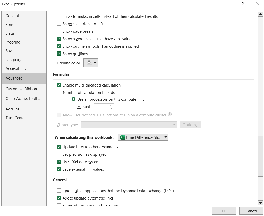
In the Excel Options dialog box, click Advanced.
-
Scroll down to the When calculating this workbook section.
-
Check the box labeled Use 1904 date system, and click OK.
-
Enter your time values as usual—in this case, A2 and B2.
-
Subtract the times to find the difference using this method. In cell C2, type
=B2-A2, and press Enter. -
Then, you can format the result as a time. In the Format Cells dialog box in the top menu, go to the Number tab, select Custom, and use the time format [h]:mm:ss or any other format that suits your needs.

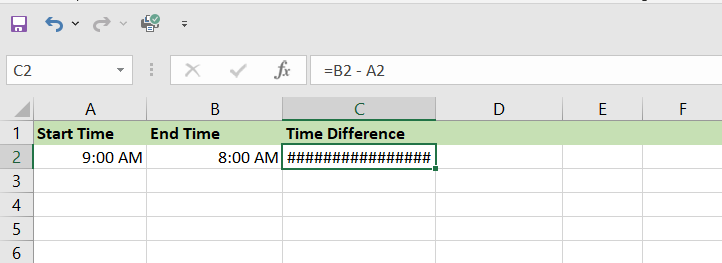
For reference, here’s what that same formula looks like without the 1904 date system applied.
Converting time differences to specific units
You can convert any given time difference to hours, minutes, or seconds using one of the following formulas. The process for conversion is the same for each.
-
Hours:
=(End time - Start time) * 24 -
Minutes:
=(End time - Start time) * 1440 -
Seconds:
=(End time - Start time) * 86400
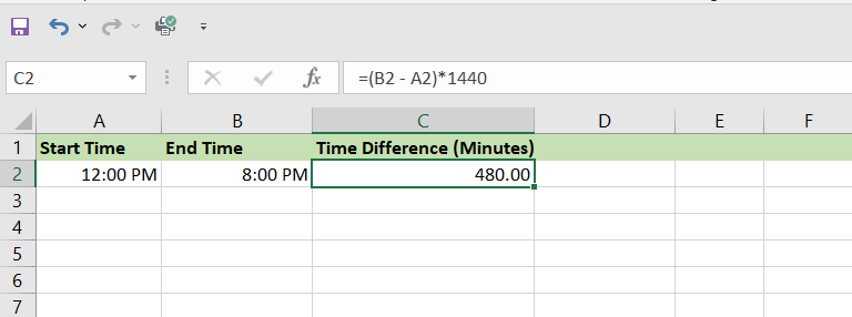
I’ll quickly walk you through the steps for converting time differences to specific units here. In this example, we’ll calculate the minutes.
-
Enter your time values as usual—in this case, A2 and B2.
-
Click on the cell where you want the result—for example, C2.
-
Type the formula:
=(End time - Start time) * 24. For this example, we’ll use:=(B2 - A2)*1440. Then, press Enter.
Using the TEXT function for time differences
The TEXT function in Excel is another tool you can use for time differences: it allows you to convert a numeric value to text in a specified format. This really isn’t the most efficient way to work with time in Excel, but you do you.
-
Enter your time values as usual—in this case, A2 and B2.
-
Click on the cell where you want the result—for example, C2.
-
Type the formula:
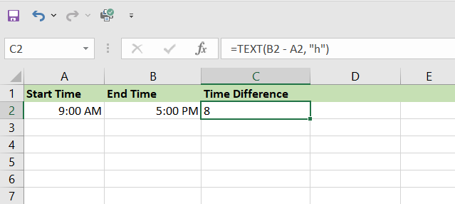
=TEXT(End time - Start time, "h"). In this example, this will read=TEXT(B2 - A2, "h"). -
Hit Enter. The difference in the number of hours will appear in the selected cell.
You can also do the same thing with the following time-related text functions:
-
Hours:
=TEXT(End time - Start time, "h") -
Hours and minutes:
=TEXT(End time - Start time, "h:mm") -
Hours, minutes, and seconds:
=TEXT(End time - Start time, "h:mm:ss")
Formulas for time calculation in Excel
That’s enough screenshots of my Excel instance. It’s your turn now. Check out the table below to grab your formula and go.
|
Name |
Formula |
|---|---|
|
Basic time difference |
|
|
Time difference in hours |
|
|
Time difference in minutes |
|
|
Time difference in seconds |
|
|
Using the TEXT function to format time differences |
Hours only
Hours and minutes
Hours, minutes, and seconds
|
|
Calculating elapsed time from a start time to now |
|
Tricks for working with time values in Excel
There are some general principles beyond just getting your formulas right that can help steer your sheets clear of any time difference calculation mishaps. Think of these less as steps to follow and more as…learning from my mistakes.
-
Use consistent formatting: Make sure you’re adding all time values using Excel’s Time or Date/Time formats. This is not the time for creative license.
-
If there’s a built-in function, use it: Excel is full of built-in time functions like TODAY(), NOW(), and more that can deliver accurate time data in the blink of an eye. For example, if you enter TODAY() in a cell and hit Enter, Excel will automatically fill in today’s date.
-
Avoid text entries: I know I said you can use the TEXT function earlier, but honestly, I recommend against it. It overcomplicates the process. Excel is designed to work with numbers, so it will perform best when you give it those numbers and format them as such.
-
Use data validation: If you want to be fancy, you can restrict entries in certain cells to certain formats with data validation. This will force you or other sheet users to avoid entering times as text. Just follow this path: Data > Data Validation > Settings, then choose Time and set the desired conditions.
Automate Excel with Zapier
There’s definitely a time and place for a manual process—but if I could automatically convert all the timestamps on my Denver coworkers’ messages, I absolutely would.
You can use Zapier to automate Excel processes across thousands of apps to automatically pull data into Excel or send it to the other tools you use most. Learn more about how to automate Excel, or get started with one of these pre-made workflows.
Zapier is a no-code automation tool that lets you connect your apps into automated workflows, so that every person and every business can move forward at growth speed. Learn more about how it works.
Related reading: