Interpreting spreadsheets full of data isn’t a skill that comes naturally to me. My eyes glaze over from information overload before I can even get into the meat and potatoes of what it all means. That’s why I use conditional formatting.
It helps me better understand key data at a glance so I can track things like my spending habits and how my team is progressing toward our quarterly goals.
Here, I’ll walk you through the basics of conditional formatting in Google Sheets. And I’ll show you how to apply some of the most common formatting rules. To follow along, use our demo spreadsheet. Copy the spreadsheet, and then play around with it as we proceed through the tutorial.
But first, if you’re looking for a quick refresher, here’s the short version on how to use conditional formatting. (Scroll down to learn more specifics and practice with our demo spreadsheet.)
-
Highlight the cell range you want to apply the formatting rules to.
-
Select Format > Conditional formatting.
-
From the Conditional format rules window that appears, click the dropdown menu under Format cells if…
-
Select the condition you want to trigger your rule.
-
Under Formatting style, select your formatting style.
-
Click Done.
Want to view all the rules in your spreadsheet? Simply highlight the entire data range (or the whole sheet), and open the Conditional format rules window using the first step from above. This will display a complete list of any existing rules. You can also quickly delete any rules by selecting the Remove rule icon, which looks like a garbage can.
What is conditional formatting in Google Sheets?
In Google Sheets, conditional formatting allows you to dynamically change a cell’s text style and background color based on custom rules you set. Every rule you set is created using an if this, then that statement.
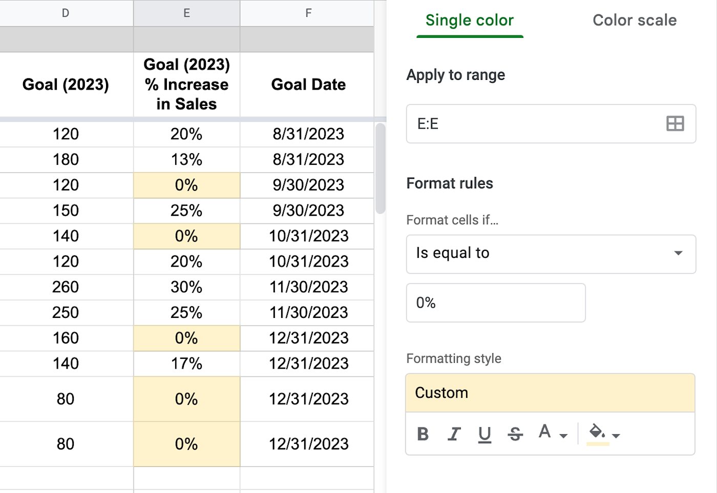
In the example below, the rule tells Google Sheets, “If any cell in column E is equal to 0%, then change that cell’s background color to light yellow.”
Before we go further, let’s clarify the three key components that make up every conditional formatting rule.
-
Range: The cell (or cells) which the rule applies to. In the example above, the range is “E:E” (i.e., all of column E).
-
Condition: This is the “if” part of the if this, then that rule. It refers to the trigger event that needs to happen for the rule to run. In the example above, the condition is “is equal to.”
-
Formatting: This is the “then” part of the if this, then that rule. It refers to the formatting that should apply to any given cell, if the conditions are met. In the example above, the style is “background color to light yellow.”
If you’ve used Zapier before, the rules of conditional formatting might sound familiar. It works a lot like a Zap (what we call our automated workflows): if the trigger event happens, then the action will follow.
How to do conditional formatting in Google Sheets
Conditional formatting is an efficient way to make valuable information stand out. Here’s how to create and modify conditional formatting rules in Google Sheets.
1. Select a range
First, select your desired range. You can do this one of two ways.
Option 1: Highlight a range directly in the spreadsheet. This can be anything from a single cell to multiple cells across different rows and columns. If you’re not managing a lot of data, this is the quickest way to go.
Option 2: Without highlighting anything, select Format > Conditional formatting. From the Conditional format rules window that appears, enter your desired range under Apply to range.
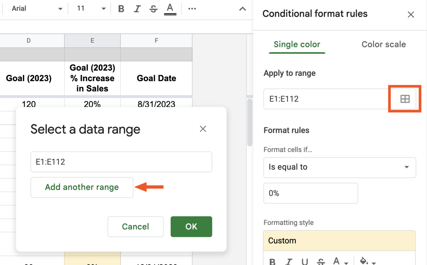
To add more ranges, click Select data range, which looks like a grid, from the cell range text box. In the Select a data range window that appears, click Add another range.
2. Create the condition
Once you’ve selected your range, create your trigger rule (i.e., your if this, then that statement) in the Format cells if section. There are a lot of triggers to choose from, which will impact how you format your rule. Let’s look at the most common triggers.
Tip: If you select Conditional formatting, but you haven’t applied any conditional formatting rules to the selected range, Google Sheets will automatically add a default rule for you: “if cell is not empty, change the background color to light green.” But you can easily edit this (scroll to the bottom of this article to find out how). If you’ve already applied rules to the given range, these will appear in the Conditional format rules window.
Apply conditional formatting with is empty/is not empty
The first set of triggers—cell is empty and cell is not empty—will run based on whether or not there’s data in the specified range.
Try it out:
-
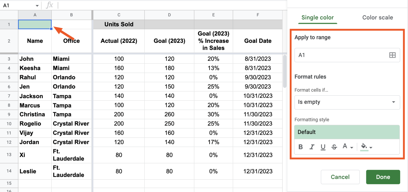
In the demo spreadsheet, select cell
A1, and then click Format > Conditional formatting. -
Select the trigger is empty. Since the selected cell (
A1) is empty, the default conditional formatting will apply. Magic! (Note: not actually magic.)
Tip: To remove a conditional formatting rule, select any cell that’s been included in the rule, and then open the Conditional format rules window. A list of applied rules will appear. Select the Remove rule icon, which looks like a garbage can, to delete the rule.
Apply conditional formatting based on text
To automatically format a cell based on its text, use any of these text-based triggers:
-
Text contains
-
Text does not contain
-
Text starts with
-
Text ends with
-
Text is exactly
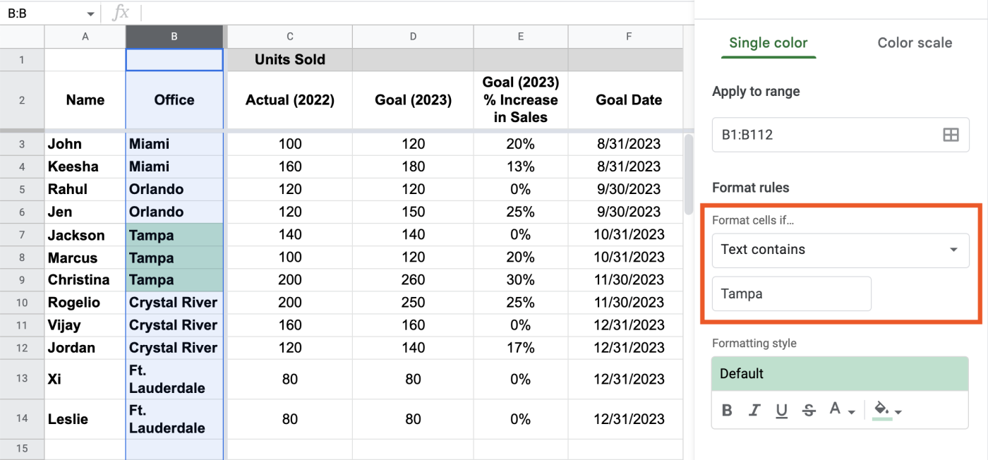
Try it out: Let’s say you want to highlight all of your employees based in the Tampa office.
-
Select column B, and click Format > Conditional formatting.
-
Under Format cells if, select Text contains.
-
In the Value or formula field, enter
Tampa(the text value isn’t case sensitive).
Now, the default formatting style will apply to any cell containing the word “Tampa.” And since you applied the rule to all of column B, any time you add a new rep in the Tampa office, the cell containing “Tampa” will automatically be highlighted for easy access.
Apply conditional formatting based on number values
To automatically format a cell based on numbers, use any of these triggers:
Try it out: Let’s say you want to highlight “stretch” goals i.e., any goals where the increase is 20% or higher.
-
Select column E, and click Format > Conditional formatting.
-
Under Format cells if, select Greater than or equal to.
-
In the Value or formula field, enter
20%.
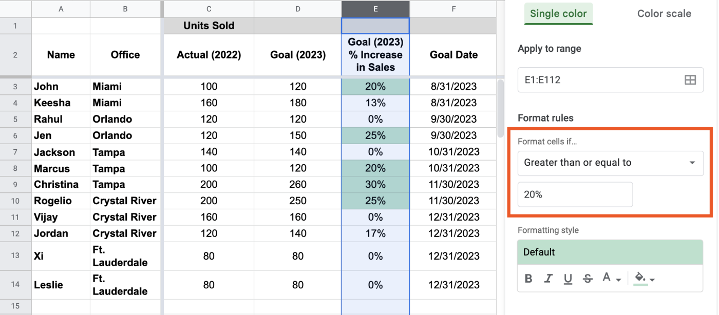
Tip: Google Sheets recognizes any type of number—from percentiles to currencies. This is especially useful if you want to track anything from your monthly spending habits to the percentage of your business goals achieved.
Apply conditional formatting to an entire row
Let’s kick things up a notch and apply conditional formatting to entire rows. To do this, using a custom formula is your best bet.
Try it out: Let’s say you want quick access to all data associated with your existing Tampa reps, including their names and sales targets.
-
Highlight your entire data set (in this case,
A3:F14), and select Format > Conditional formatting. -
Under Format cells if, select Custom formula is (last option).
-
In the Value or formula field, enter
=$B:$B="Tampa".
Now, any row containing “Tampa” in column B is highlighted.
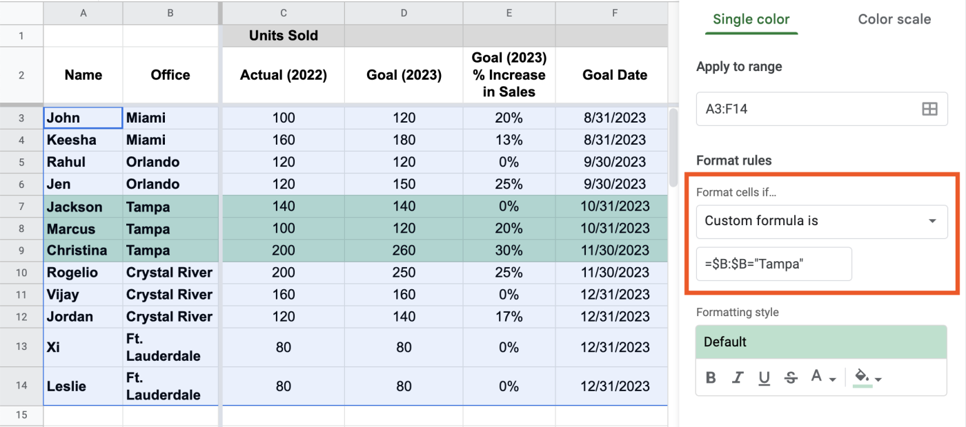
How did that work? Let’s nerd out and break the custom formula down.
The = symbol indicates the start of the formula. $B:$B tells Google Sheets to scan through column B for a specific value. By adding the $ before B, it tells Google to only scan through column B. And finally, ="Tampa" tells Google Sheets what value to look for.
Now, let’s say you want to highlight any row where the stretch goal is greater than or equal to 20%. Again, you’d use a custom formula. In this case, you would enter =$E:$E>=20%.
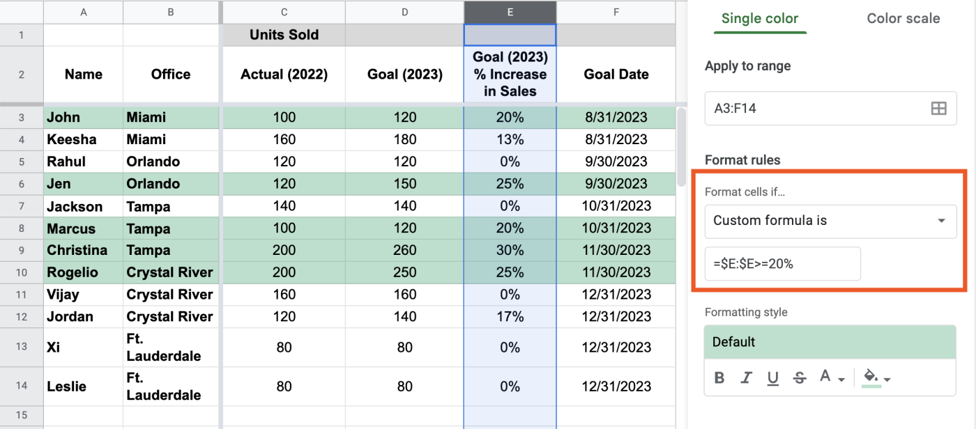
If you’re applying a custom formula based on number values, there are more operators you can play around with: less than or equal to (<=), less than (<), greater than (>), or equal to (=).
You can also use a custom formula to highlight any rows that don’t include a given value. For example, if you wanted to highlight your reps who don’t work out of the Tampa office, you’d use the custom formula =$B:$B<>"Tampa".
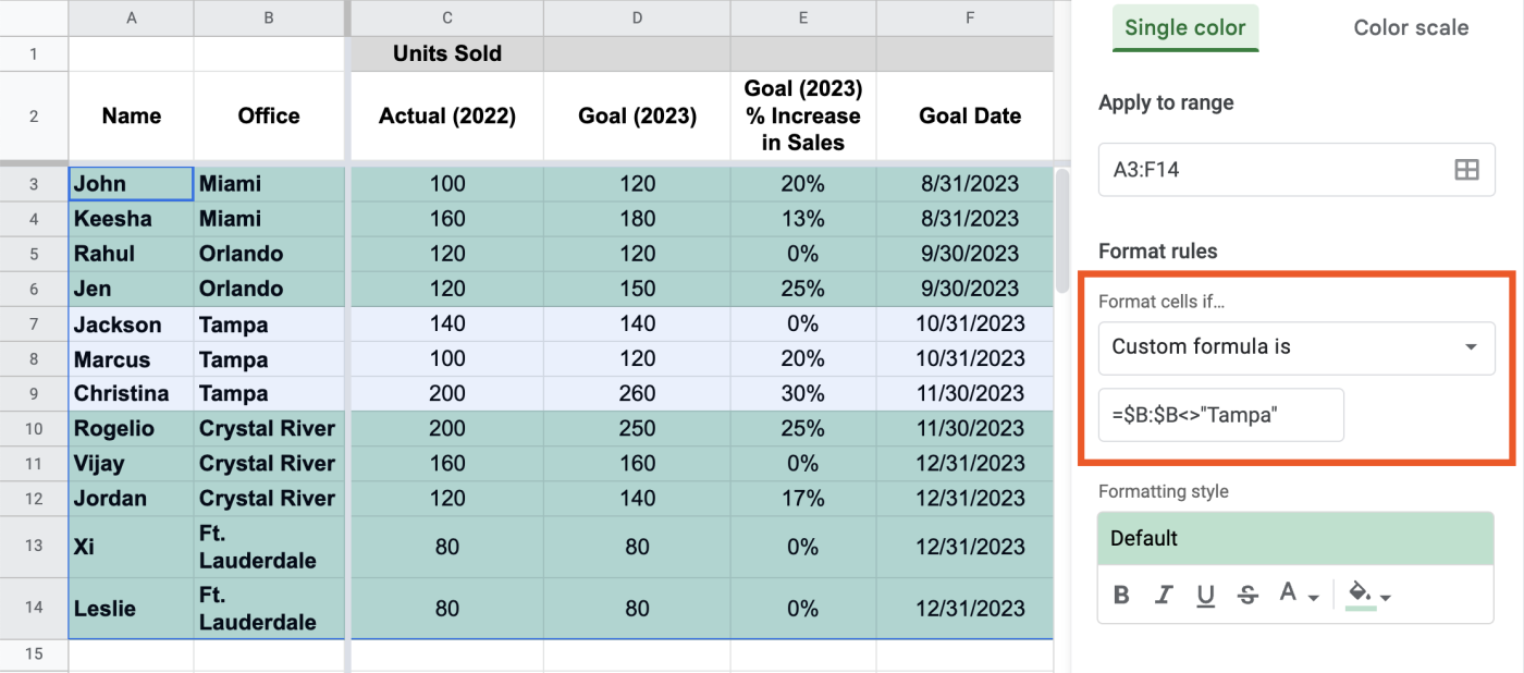
Tip: The above examples just scratch the surface of what’s possible with custom formulas. If you want to go further down the rabbit hole, check out this list of formulas accepted by Google Sheets. Heads-up: they get advanced pretty quickly.
Apply conditional formatting using a color scale
The color scale is another formatting style that makes it easier to visualize values on a spectrum.
Try it out: Let’s say you want to see where your reps’ stretch goals fall on a spectrum: a 0% increase being not great, and a 50% being “Wow! Now that’s a stretch goal.” A great way to visualize this is by using a color scale where the fill color differs in intensity based on the cell value. Here’s how.
-
Highlight column E, and then click Format > Conditional formatting.
-
In the Conditional format rules window, click Color scale. The default formatting will appear, highlighting the lowest stretch goal percentages with a highly saturated color (in this case, dark green) and the highest ones with a less saturated version of the same color (in this case, light green).
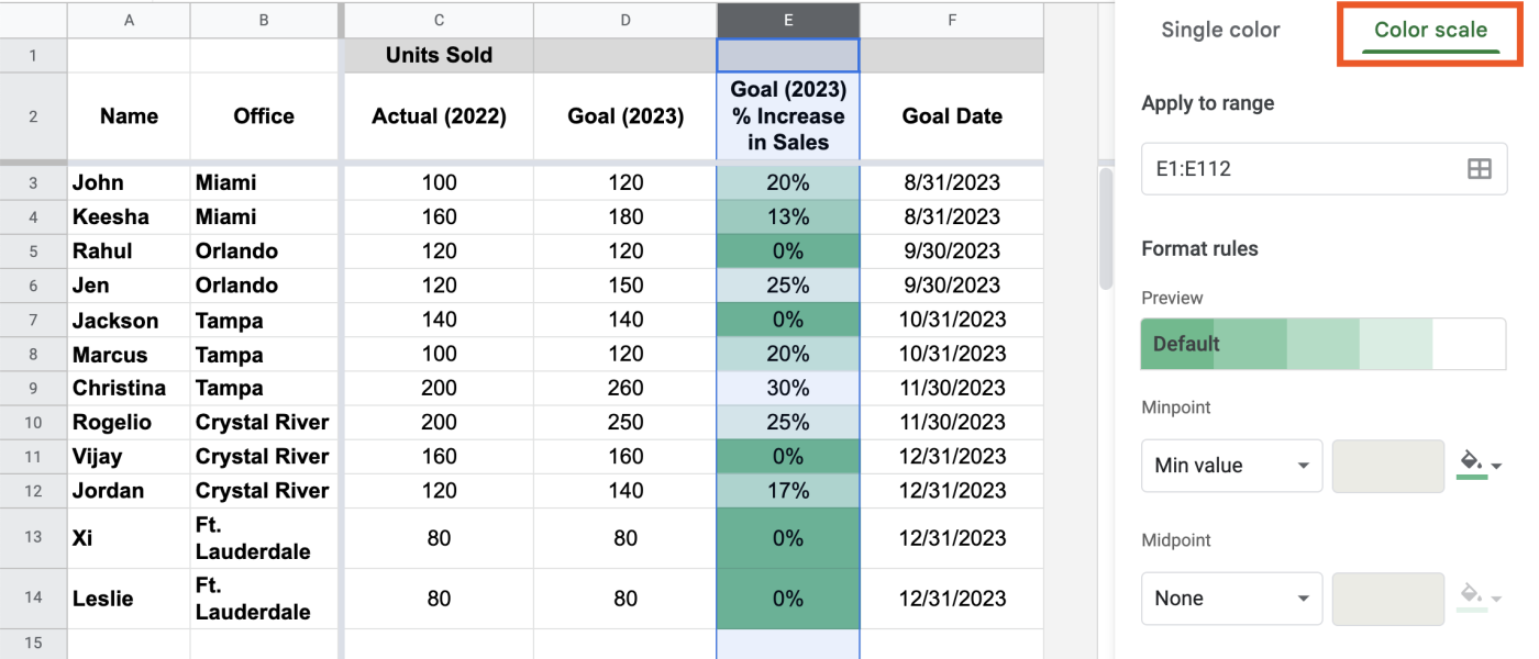
Tip: If your conditional formatting rule modifies a cell’s background color, use a high-contrast color scheme to improve readability. In the case of using a color scale, shades of yellow against a black font would be better than, say, shades of red.
Apply conditional formatting based on dates
Before applying conditional formatting rules using dates, it’s important to use a consistent date format throughout your spreadsheet.
To do this, highlight any cells that include dates, click Format > Number. From here, you can either select the default date format, or select Custom date and time and choose your preferred style.
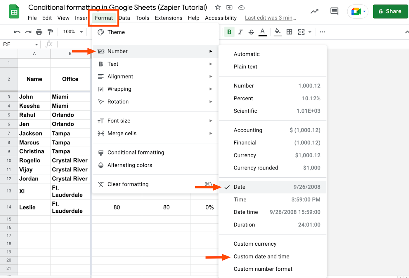
Now that your date format is consistent throughout, let’s apply some conditional formatting rules. Here are your options for date-based rules:
-
Date is
-
Date is before
-
Date is after
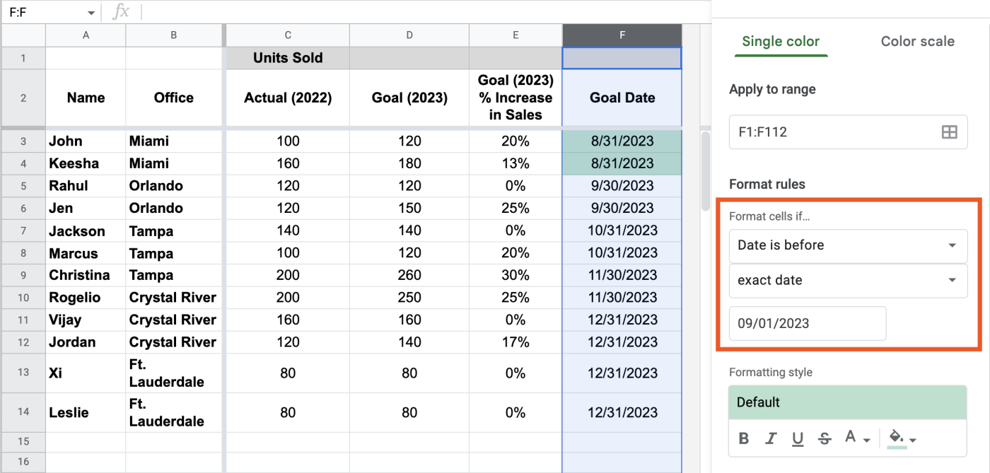
Try it out: Let’s say you want to highlight reps who have goals to increase their sales by the end of August.
-
Highlight column F, and then click Format > Conditional formatting.
-
Under Format cells if, select Date is before > Exact date.
-
In the Value or number field, enter 09/01/2023.
Tip: Use conditional formatting using relative dates, such as today, tomorrow, yesterday, and in the past week, month, or year. This way, you don’t have to keep manually updating your rules to communicate things like deadlines and goals.
Apply multiple conditional formatting rules
Adding more than one conditional formatting rule to a given range is easy. Simply highlight the range, click Format > Conditional formatting, and then click Add another rule.
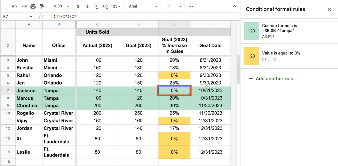
Google Sheets will run through each rule—in the order they were created—until it finds a condition that requires a style change. However, once a rule is met by any given cell, subsequent rules won’t override it.
In the example below, the following conditional formatting rules have been applied to the entire data range (A3:F14):
-
First: If the rep is based in Tampa, highlight the entire row in light green. To do this, I used the same formula from before:
=$B:$B="Tampa". -
Second: If the sales goal increase of any rep is equal to 0%, highlight the cell in light yellow. To do this, I set the rule to “is equal to 0%.”
Jackson (row 7) works from the Tampa office. Because this meets the first rule, row 7 is highlighted in green. Even though Jackson also has a 0% increase in his sales goals and the second rule theoretically applies, it doesn’t matter to Google Sheets. It’s one conditional formatting rule to… rule them all.
Tip: If you notice that your rule isn’t working as it should, it might be because it’s being blocked by another rule. Delete any previous rules applied to the same range. This should get your rule back in working order.
3. Select a formatting style
Up to this point, we’ve mainly used Google Sheets’ default formatting style to highlight specific cells. But if you want to add a little more pizzazz, you can easily update your formatting style. Here’s how.
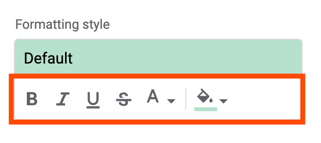
In the Conditional format rules window, click Default under Formatting style to choose from five other preset styles. If none of these options meet your needs, you can also create a custom style using the tools under Formatting style.
Tip: Humans subconsciously associate specific colors with specific meanings, so be mindful about your color choices. For example, if I used conditional formatting to highlight any data indicating that my team fell short of their quarterly targets, I wouldn’t use red. Instead, I might opt for something more neutral, but still noticeable, like orange. For more information about how to use color to your advantage, check out Canva’s guide to color meaning and symbolism.
Bonus: How to copy and paste conditional formatting to another Google Sheet
Let’s say you have multiple sheets of data, and you want to apply the same conditional formatting rules from one worksheet to another in Google Sheets. You could apply the same rules manually, or you can take a much faster route: copy and paste—but make it special. Here’s what I mean.
In the example below, there are two spreadsheets of sales data: one for 2022 goals and another for 2023 goals. In the 2022 Goals spreadsheet, the rule is “if value is equal to 0%, highlight the cell in light green.” Here’s how to apply the same rule to the 2023 Goals spreadsheet.
-
Click any cell that has the desired rule applied in the 2022 Goals spreadsheet, and use your keyboard shortcut to copy it.
-
Click the spreadsheet tab 2023 Goals.
-
Highlight the data range in column E (
E3:E14). -
Right-click, and select Paste special > Format only.
Any cells in column E with the value 0% will immediately be filled in light green.
Tip: You can only copy and paste conditional formatting rules from one worksheet to another if the value types are the same. For example, you can’t copy a rule that applies to whole numbers and paste it to cells containing percentages.
Related reading
This article was originally published in December 2018 by Theodor Porutiu. The most recent update was in June 2024.